Refined Products Distribution

Batch scheduling, the Cola equation for transmix volume, and terminal inventory design from Edmonton to Burnaby

pipelines
refined products
batch scheduling
dispersion
energy
Alberta
A litre of diesel refined at Edmonton’s Strathcona Refinery reaches a Vancouver pump in roughly nine days, sharing a pipeline with gasoline and jet fuel, separated by mathematics. This article derives the dispersion equation governing contamination at batch interfaces, works through the scheduling logic that sequences incompatible products safely, and builds the terminal inventory model that keeps Metro Vancouver supplied across a transit time that cannot be shortened by wishing.
Published

May 12, 2026

Part of the Alberta Pipeline Geography cluster. This is P4 of five articles. P1 — Crude Oil Pipelines · P2 — NGL and Condensate Systems · P3 — Natural Gas Transmission · P5 — The Integrated Network


Before You Start

You should know Basic probability and statistics: what a normal distribution is, what a standard deviation measures. The Darcy-Weisbach equation from P1 (friction factor, Reynolds number) — the same turbulent friction concepts reappear here. That different liquid fuels can contaminate one another if mixed.

You will learn Why pipelines carry multiple products simultaneously rather than dedicating separate pipes to each fuel; how turbulent dispersion inevitably mixes the boundary between adjacent batches; how G.I. Taylor’s 1954 dispersion theory produces the quantitative equation for that mixing; the sequencing rules that minimise contamination risk at aviation fuel interfaces; and how a terminal’s required inventory is an algebraic function of the pipeline’s transit time, the batch delivery schedule, and the demand rate. The last of these links the physics of the 1,147-kilometre Trans Mountain products line directly to the size of the tanks at Burnaby.

Why this matters The Burnaby terminal stocks approximately thirteen days of Metro Vancouver’s petroleum supply (Trans Mountain Corporation 2024). That number is not arbitrary — it is the solution to an inventory design equation whose inputs include the nine-to-ten-day pipeline transit time derived from the Darcy-Weisbach hydraulics of P1. A prolonged shutdown of the Trans Mountain products pipeline (as happened in November 2018 during a spill response and in subsequent maintenance outages) draws down those thirteen days of inventory faster than alternative supply can be established. Understanding why the buffer is sized as it is requires tracing through the same physical equations that govern how much diesel can move through a 20-inch pipe per day.

If this gets hard, focus on… The Cola equation’s key result is that interface contamination grows as the square root of pipeline distance. A pipeline twice as long doesn’t produce twice as much transmix — it produces \sqrt{2} \approx 1.41 times as much. This is the direct consequence of diffusion being a random-walk process. Everything else in this article builds from that one scaling relationship.


The Strathcona Refinery sits on the south bank of the North Saskatchewan River, roughly ten kilometres east of downtown Edmonton. Its crude oil arrives by Enbridge Mainline; its products depart by three routes: truck rack for local Alberta distribution, the Puget Sound pipeline for northward BC interior delivery, and the Trans Mountain products pipeline for the 1,147-kilometre journey to Burnaby (Imperial Oil Limited 2024). At any given moment, the Trans Mountain products pipe contains roughly eight batches of different fuels in sequence, each batch a cylinder of fluid occupying some fraction of the pipe’s 200,000-barrel working inventory. Premium gasoline follows regular gasoline, which follows diesel, which buffers jet fuel, which yields back to diesel before the gasoline cycle repeats. The sequence is not arbitrary. It is the solution to a scheduling and contamination-management problem that the mathematics of turbulent flow makes precise.

At the Burnaby terminal on Burrard Inlet, tank farm operators know exactly when each batch will arrive. They calculated it from the injection time at Edmonton, the pipeline flow rate, and the 1,147-kilometre pipe length. They are right to within a few hours. They maintain 13 days of storage not because that is a regulatory requirement but because that is the algebraic consequence of a 9.5-day transit time, a normal batch cycle, and a safety buffer that covers the most likely disruption duration. The pipeline’s physics determined the tank farm’s size.


1. The Question

Three connected questions drive this article:

First: why does a single pipeline carry multiple products, and how are the batches sequenced to minimise quality risk?

Second: how much contamination occurs at the interface between adjacent batches, and what equation governs the contamination volume as a function of pipe geometry, flow conditions, and distance?

Third: given that pipeline deliveries arrive in discrete batches with a known transit delay, what is the minimum terminal inventory required to guarantee supply continuity?

These are an operations question, a fluid mechanics question, and an inventory management question. They share one input: the pipeline transit time, which is determined by the hydraulics of P1.


2. The Conceptual Model

Why Multi-Product Pipelines?

Dedicated pipelines — one pipe per product — would eliminate all contamination risk. They would also be economically absurd. A 20-inch pipeline costs roughly the same whether it carries one product or five; the pipe steel, the right-of-way, the pump stations, and the regulatory approvals are fixed costs per kilometre. The Trans Mountain products pipeline, if replicated as five dedicated lines (gasoline, diesel, jet fuel, heating oil, aviation gasoline), would require five times the capital for roughly the same throughput. The capital cost of product segregation is the cost of four additional 1,147-kilometre pipelines.

Instead, products share the pipe sequentially. Each product travels as a discrete batch — a plug of fluid, typically 20,000 to 300,000 barrels, moving at the same velocity as the rest of the fluid in the pipe. Because fluid in a circular pipe moves as an approximately plug-flow (the velocity profile across the cross-section is turbulently flattened, not the parabolic laminar profile of low-Reynolds-number flow), the batch identity is largely preserved during transit. Largely — but not completely.

Why Transmix Occurs

At the boundary between two adjacent batches, the interface is not infinitely sharp. At injection, the upstream batch ends and the downstream batch begins over roughly the transition distance of the injection valve — centimetres. But as the fluid travels, two mixing mechanisms broaden that interface:

Molecular diffusion is negligible in turbulent pipeline flow. Molecular diffusivity of hydrocarbon mixtures is approximately 10^{-9} m²/s. Over a 1,147-kilometre transit at 1.4 m/s (roughly 9.5 days), molecular diffusion alone would spread the interface by \sigma \approx \sqrt{2 D_{mol} t} = \sqrt{2 \times 10^{-9} \times 820{,}000} \approx 0.04 m — negligible.

Turbulent dispersion is the dominant mechanism. Even in plug-flow conditions, turbulent eddies laterally mix fluid parcels across the pipe cross-section. A fluid element near the pipe wall moves slightly slower than one at the centreline (the velocity profile is nearly flat but not perfectly so). Over time, this velocity gradient — even the small residual gradient in turbulent flow — shears the interface longitudinally, producing an elongated mixing zone. G.I. Taylor’s (1954) analysis of this mechanism showed that the net effect is equivalent to longitudinal diffusion with an apparent diffusivity many orders of magnitude larger than molecular diffusion (Taylor 1954).

The transmix — the mixed-product interface volume that falls outside specification for both products — must be diverted to reprocessing tankage at the receiving terminal, blended into the lower-specification product at a discount, or re-injected as an interface slug into the pipe for the next cycle. Managing its volume is the central engineering problem of refined products pipeline operations.


3. Building the Mathematical Model

3.1 Turbulent Dispersion: Taylor’s Theory

Taylor (1954) showed that in turbulent pipe flow, the random action of turbulent eddies produces an apparent longitudinal dispersion coefficient K (Taylor 1954):

K = 10.1 \, r_0 \, u^*

where: - r_0 = D/2 — pipe radius [m] - u^* = v\sqrt{f/8} — shear velocity [m/s], with v the mean flow velocity and f the Darcy friction factor

The shear velocity u^* measures the intensity of turbulence near the wall — it is the velocity scale associated with the wall shear stress \tau_w = \rho (u^*)^2. Higher velocity and rougher pipe produce larger u^* and larger K.

Physical meaning: K plays the role of a diffusivity, but its magnitude is determined by turbulent mixing rather than molecular motion. For a 20-inch products pipeline at typical operating conditions:

  • v \approx 1.4 m/s, D = 0.508 m
  • f \approx 0.013 (turbulent, commercial steel pipe)
  • u^* = 1.4 \times \sqrt{0.013/8} = 1.4 \times 0.0403 = 0.0564 m/s
  • K = 10.1 \times 0.254 \times 0.0564 = 0.145 m²/s

Compare to molecular diffusivity of 10^{-9} m²/s: turbulent dispersion is approximately 145 million times more effective at longitudinal mixing than molecular diffusion. This is why ignoring molecular diffusion in pipeline batch analysis is perfectly valid, while ignoring turbulent dispersion is not.

3.2 The Interface Concentration Profile

Taylor’s theory predicts that a sharp initial interface between two miscible fluids evolves, at position x from the injected interface after travelling distance L at mean velocity v, as:

c(x) = \frac{1}{2} \operatorname{erfc}\!\left(\frac{x}{\sqrt{2}\,\sigma_x}\right)

where \operatorname{erfc} is the complementary error function and \sigma_x is the spatial standard deviation of the concentration profile:

\sigma_x = \sqrt{\frac{2KL}{v}}

This is the dispersion analogue of the standard deviation growth in Brownian motion: the interface width grows as L^{1/2}, not linearly with distance. This square-root scaling is the mathematical statement that diffusion is a random-walk process — each step adds in quadrature, not in sum.

At x = 0: c = 0.5 (equal parts of both products — the centreline of the interface). At x = +\infty: c = 0 (pure downstream product). At x = -\infty: c = 1 (pure upstream product).

For a concentration cutoff c_{\text{cut}} defining the edge of the “contaminated” zone, the half-width of the transmix region is:

x_{\text{cut}} = \sqrt{2}\,\sigma_x \cdot \operatorname{erfinv}(1 - 2c_{\text{cut}})

where \operatorname{erfinv} is the inverse error function. For the 1–99% contamination band (c_{\text{cut}} = 0.01): \operatorname{erfinv}(0.98) \approx 1.645, so x_{1\%} = 1.645\sqrt{2}\,\sigma_x = 2.326\,\sigma_x.

3.3 The Cola Equation for Transmix Volume

The total transmix volume between the c_{\text{cut}} concentration cutoffs on each side of the interface is:

V_{mix} = A \cdot 2 x_{\text{cut}} = A \cdot 4.652\,\sigma_x \quad \text{(for the 1–99\% band)}

where A = \pi D^2/4 is the pipe cross-sectional area. Substituting \sigma_x = \sqrt{2KL/v} and K = 10.1\,(D/2)\,v\sqrt{f/8}:

\sigma_x = \sqrt{\frac{2 \times 10.1 \,(D/2)\,v\sqrt{f/8}\,L}{v}} = \sqrt{10.1\, D\, L\, \sqrt{f/8}}

Combining with A = \pi D^2/4:

\boxed{V_{mix} = 4.652 \cdot \frac{\pi D^2}{4} \cdot \sqrt{10.1\,D\,L\,\sqrt{f/8}} = 6.91\, f^{1/4}\, D^{5/2}\, L^{1/2}}

where all quantities are in SI units (m³, m, m). This result — the Cola equation (Cola 1965; Menon 2015) — gives the 1–99% transmix volume in terms of pipe diameter, pipe length, and friction factor. The diameter exponent 5/2 = 2.5 and length exponent 1/2 = 0.5 are the defining scaling relationships.

Converting to field units (V in barrels, D in inches, L in miles, f = 0.013):

V_{mix} = 0.0606 \cdot D^{2.5} \cdot L^{0.5} \quad \text{(bbl, in, mi, at } f = 0.013\text{)}

The f-dependence is mild — f^{1/4} — so a 50% increase in friction factor changes transmix by only 1.5^{0.25} - 1 = 11\%. Pipe diameter and distance are the dominant design variables.

3.4 Minimum Batch Size

The practical consequence of the Cola equation is a minimum batch size: a batch must be large enough that the transmix volumes at each interface consume only a modest fraction of the total batch, leaving sufficient on-specification product to meet contracted delivery.

If a batch of product X has transmix interfaces on both the leading and trailing edges (upstream product and downstream product each contaminating one interface), the minimum batch volume to deliver V_{\text{delivery}} of on-specification product is:

V_{\text{batch}} = V_{\text{delivery}} + V_{\text{mix,lead}} + V_{\text{mix,trail}}

For symmetric interfaces (both interfaces have the same Cola volume):

V_{\text{batch}} = V_{\text{delivery}} + 2\,V_{mix}

The fraction of each batch consumed by transmix is called the interface loss ratio:

\eta_{mix} = \frac{2\,V_{mix}}{V_{\text{batch}}} = \frac{2\,V_{mix}}{V_{\text{delivery}} + 2\,V_{mix}}

For the Trans Mountain products line (20-inch pipe, 1,147 km), V_{mix} \approx 2{,}900 bbl per interface. A typical diesel batch of 60,000 bbl delivers approximately 60{,}000 - 2 \times 2{,}900 = 54{,}200 bbl of on-specification fuel. The interface loss ratio is 5{,}800 / 60{,}000 \approx 9.7\%. For a 200,000 bbl batch, the ratio falls to 5{,}800 / 200{,}000 \approx 2.9\%. Larger batches are more efficient, which is why products pipelines prefer infrequent large batches over frequent small ones, subject to the constraint that batch cycle time must not force excessive terminal inventory buildup.

3.5 Terminal Inventory Design

A receiving terminal at the end of a pipeline is not a simple tank — it is an inventory buffer calibrated to the pipeline’s physics. Its required storage capacity follows from a simple balance.

Let: - D_d — average daily demand [m³/day] at the terminal - t_{transit} — pipeline transit time [days] = L/v - t_{cycle} — average time between deliveries of the same product [days] - t_{safe} — safety stock [days] (coverage for demand spikes and pipeline disruption)

The terminal’s working inventory must be able to absorb the full demand during one complete delivery cycle without a stockout, even if the next scheduled batch is delayed by t_{safe} days:

\boxed{V_{working} = D_d \times (t_{cycle} + t_{safe})}

The transit time t_{transit} does not appear in the working inventory formula directly — it appears instead as the reorder lead time: the pipeline operator must inject the next batch t_{transit} days before the terminal needs it, so that the batch arrives on time.

The total design inventory (maximum storage required) must accommodate the full transit delay plus the safety buffer — the tank must not run dry during the worst-case scenario of a new batch delayed by both the full transit time and the safety period:

V_{\text{design}} = D_d \times (t_{transit} + t_{cycle} + t_{safe})

For the Burnaby terminal serving Metro Vancouver diesel demand: - D_d \approx 8{,}000 m³/day - t_{transit} = 9.5 days - t_{cycle} \approx 1.5 days (time between diesel injections in a rotating multi-product schedule) - t_{safe} = 2 days

V_{\text{design}} \approx 8{,}000 \times (9.5 + 1.5 + 2) = 8{,}000 \times 13 = 104{,}000 \;\text{m}^3

The hub article states that the Burnaby terminal maintains “approximately thirteen days” of supply — the (9.5 + 1.5 + 2) = 13 days total is not coincidental. The transit time, the batch cycle, and the safety buffer add arithmetically to the storage requirement.


4. Worked Example by Hand

Scenario: Calculate the transmix volume at the diesel/jet fuel interface on the Trans Mountain products pipeline, determine the minimum batch size for a contracted jet fuel delivery of 45,000 barrels, and size the Burnaby jet fuel tank.

Given parameters:

Parameter Value
Pipe inner diameter D 0.508 m (20 inches)
Pipeline length L 1,147,000 m (1,147 km)
Mean flow velocity v 1.40 m/s
Darcy friction factor f 0.013 (turbulent, commercial steel)
Contracted jet fuel delivery 45,000 bbl = 7,155 m³
Jet fuel daily demand (YVR) 2,000 m³/day
Safety stock 3 days (aviation fuel; stricter than road fuels)
Batch cycle time 4 days (jet fuel delivered once per 4-day cycle)

Step 1 — Dispersion coefficient

K = 10.1 \times (D/2) \times v\sqrt{f/8} = 10.1 \times 0.254 \times 1.40 \times \sqrt{0.013/8}

= 10.1 \times 0.254 \times 1.40 \times 0.0403 = 0.1447 \;\text{m}^2/\text{s}

Step 2 — Interface standard deviation

\sigma_x = \sqrt{\frac{2KL}{v}} = \sqrt{\frac{2 \times 0.1447 \times 1{,}147{,}000}{1.40}} = \sqrt{\frac{331{,}918}{1.40}} = \sqrt{237{,}084} = 487 \;\text{m}

The interface is approximately 487 m wide in standard deviation terms — about half a kilometre of pipe length.

Step 3 — Transmix volume (1–99% band)

V_{mix} = 4.652 \times A \times \sigma_x = 4.652 \times \frac{\pi (0.508)^2}{4} \times 487

= 4.652 \times 0.2027 \times 487 = 459 \;\text{m}^3 = 2{,}888 \;\text{bbl}

Or equivalently, from the Cola equation: V_{mix} = 6.91 \times (0.013)^{0.25} \times (0.508)^{2.5} \times (1{,}147{,}000)^{0.5} = 6.91 \times 0.3376 \times 0.1839 \times 1{,}070.8 = 459 \;\text{m}^3 \;\checkmark

The diesel/jet fuel interface produces approximately 460 m³ (2,900 bbl) of transmix per interface. Because the jet fuel batch has a diesel buffer on both sides (see Section 6), the batch has two diesel/jet interfaces and one jet/diesel interface on the trailing edge — effectively three Cola volumes to manage.

Step 4 — Minimum jet fuel batch size

The contracted delivery is 45,000 bbl = 7,155 m³. Including interfaces:

V_{\text{batch}} = V_{\text{delivery}} + 2 \times V_{mix} = 7{,}155 + 2 \times 459 = 8{,}073 \;\text{m}^3 \approx 50{,}800 \;\text{bbl}

The pipeline must inject 50,800 bbl to deliver 45,000 bbl — a transmix allowance of approximately 11%.

Step 5 — Jet fuel tank design at Burnaby

V_{\text{design}} = D_d \times (t_{transit} + t_{cycle} + t_{safe}) = 2{,}000 \times (9.5 + 4 + 3) = 2{,}000 \times 16.5 = 33{,}000 \;\text{m}^3

Approximately 210,000 bbl of jet fuel storage required at Burnaby — roughly three or four large aviation fuel tanks of 50,000–75,000 bbl each. This matches the scale of what Trans Mountain operates at the Burnaby marine terminal serving Vancouver International Airport via a dedicated aviation fuel line.

The stricter aviation safety stock (t_{safe} = 3 days vs. 2 days for road fuels) reflects the consequence of stockout: an aircraft unable to refuel has more immediate safety implications than a truck running low on diesel.


5. Computational Implementation

import numpy as np
import matplotlib.pyplot as plt
from scipy.special import erfc, erfinv

# ── Parameters ─────────────────────────────────────────────────────────────────
D   = 0.508       # inner diameter [m]  (20 inches)
v   = 1.40        # mean velocity [m/s]
f   = 0.013       # Darcy friction factor
L_total = 1_147_000.0  # pipeline length [m]
A   = np.pi * D**2 / 4

r0  = D / 2
u_star = v * np.sqrt(f / 8.0)
K   = 10.1 * r0 * u_star        # dispersion coefficient [m²/s]

fig, (ax1, ax2) = plt.subplots(1, 2, figsize=(13, 5.5))

# ── Left: concentration profiles at different distances ────────────────────────
distances_km = [50, 300, 700, 1147]
colours_dist = ['#3498db', '#e67e22', '#8e44ad', '#c0392b']
x_range_m = np.linspace(-2500, 2500, 2000)   # centred on interface

for L_km, col in zip(distances_km, colours_dist):
    L_m = L_km * 1000.0
    sigma_x = np.sqrt(2.0 * K * L_m / v)
    c = 0.5 * erfc(x_range_m / (np.sqrt(2.0) * sigma_x))
    ax1.plot(x_range_m / 1000.0, c, color=col, linewidth=2.0,
             label=f'{L_km} km  (σ = {sigma_x:.0f} m)')

# Mark 1-99% and 5-95% bands at 1147 km
sigma_full = np.sqrt(2.0 * K * L_total / v)
x_99 = np.sqrt(2.0) * sigma_full * erfinv(0.98)   # 1-99%
x_95 = np.sqrt(2.0) * sigma_full * erfinv(0.90)   # 5-95%

ax1.axvspan(-x_99/1000, x_99/1000, alpha=0.06, color='#c0392b',
            label=f'1–99% band: ±{x_99:.0f} m')
ax1.axvspan(-x_95/1000, x_95/1000, alpha=0.10, color='#e67e22',
            label=f'5–95% band: ±{x_95:.0f} m')
ax1.axhline(0.01, color='#95a5a6', linestyle=':', linewidth=0.8)
ax1.axhline(0.99, color='#95a5a6', linestyle=':', linewidth=0.8)
ax1.axhline(0.05, color='#bdc3c7', linestyle=':', linewidth=0.8)
ax1.axhline(0.95, color='#bdc3c7', linestyle=':', linewidth=0.8)
ax1.axhline(0.5,  color='#7f8c8d', linestyle='--', linewidth=0.7)

ax1.set_xlabel('Distance from interface centroid [km]', fontsize=10)
ax1.set_ylabel('Concentration of leading product', fontsize=10)
ax1.set_title('Interface Concentration Profile\nDiesel → Jet A on Trans Mountain (20-in, v = 1.40 m/s)',
              fontsize=11, pad=8)
ax1.legend(fontsize=8, loc='upper right')
ax1.grid(alpha=0.3)
ax1.set_xlim(-2.5, 2.5)
ax1.set_ylim(-0.02, 1.02)

# ── Right: transmix volume vs distance for three diameters ─────────────────────
L_range_km = np.linspace(10, 1400, 400)
L_range_m  = L_range_km * 1000.0

diameters  = [0.508, 0.610, 0.762]   # 20, 24, 30 inches
diam_labels = ['20 in (0.508 m)', '24 in (0.610 m)', '30 in (0.762 m)']
diam_colours = ['#2980b9', '#27ae60', '#e74c3c']

for D_i, lbl, col in zip(diameters, diam_labels, diam_colours):
    A_i   = np.pi * D_i**2 / 4
    r0_i  = D_i / 2
    u_i   = v * np.sqrt(f / 8.0)
    K_i   = 10.1 * r0_i * u_i
    sigma_i = np.sqrt(2.0 * K_i * L_range_m / v)
    # 1-99% band volume [m³]
    V_mix = A_i * 4.652 * sigma_i
    V_bbl = V_mix * 6.2898
    ax2.plot(L_range_km, V_bbl, color=col, linewidth=2.2, label=lbl)

# Mark design point
sigma_des = np.sqrt(2.0 * K * L_total / v)
V_des_bbl = A * 4.652 * sigma_des * 6.2898
ax2.plot(L_total / 1000, V_des_bbl, 'D', color='#2980b9', markersize=11,
         zorder=6, label=f'Design point: {V_des_bbl:.0f} bbl at 1,147 km')
ax2.axvline(L_total / 1000, color='#7f8c8d', linestyle='--',
            linewidth=1.0, alpha=0.7)

ax2.set_xlabel('Pipeline distance  [km]', fontsize=10)
ax2.set_ylabel('Transmix volume (1–99% band)  [bbl]', fontsize=10)
ax2.set_title('Cola Equation: Transmix Volume vs Distance\n'
              r'$V_{mix} \propto D^{2.5} \cdot L^{0.5}$',
              fontsize=11, pad=8)
ax2.legend(fontsize=9)
ax2.grid(alpha=0.3)
ax2.set_ylim(0, None)

plt.tight_layout()
plt.show()
Figure 1: Left: Concentration profile (fraction of leading product) at the diesel/jet fuel interface on the Trans Mountain products pipeline, shown at four points along the route from Edmonton to Burnaby. The interface starts as a step function and evolves according to Taylor dispersion, progressively broadening as the erfc envelope widens with the square root of distance. The 1–99% (dashed) and 5–95% (solid) transmix bands are marked at the final position (1,147 km). Right: Transmix volume (1–99% band) as a function of pipeline distance for three pipe diameters. The D^{2.5} × L^{0.5} scaling means larger pipes produce disproportionately more transmix — the 30-inch line generates 3.5× the transmix of a 20-inch line at the same distance.
import numpy as np
import matplotlib.pyplot as plt

fig, (ax1, ax2) = plt.subplots(2, 1, figsize=(11, 9))

# ── Top: pipe snapshot ────────────────────────────────────────────────────────
# Products in pipe, as fraction of total pipe length (1147 km)
# One full rotation carries 5 product types plus transmix buffers
# Approximate batch sizes (km of pipe):
batch_lengths = {
    'Premium\nGasoline': 180,
    'Regular\nGasoline': 200,
    'Diesel\n(ULSD)':    220,
    'Jet A-1\n(Aviation)': 160,
    'Diesel\n(buffer)':  170,
}
transmix_km = 1.2   # ~half a km each side, shown as 1.2 km for visibility

prod_colours = {
    'Premium\nGasoline':     '#f1c40f',
    'Regular\nGasoline':     '#e67e22',
    'Diesel\n(ULSD)':        '#2980b9',
    'Jet A-1\n(Aviation)':   '#8e44ad',
    'Diesel\n(buffer)':      '#1a5276',
}
tmx_colour = '#bdc3c7'
total_km = sum(batch_lengths.values()) + len(batch_lengths) * transmix_km * 2

x = 0.0
plot_y = 0.35
bar_h  = 0.30

# Draw batches and interfaces
for name, blen in batch_lengths.items():
    # leading transmix
    ax1.barh(plot_y, transmix_km, bar_h, left=x, color=tmx_colour,
             edgecolor='none')
    ax1.text(x + transmix_km/2, plot_y, 'tmx', ha='center', va='center',
             fontsize=6, color='#7f8c8d')
    x += transmix_km

    # product batch
    ax1.barh(plot_y, blen, bar_h, left=x, color=prod_colours[name],
             edgecolor='white', linewidth=0.5, alpha=0.88)
    ax1.text(x + blen/2, plot_y, name, ha='center', va='center',
             fontsize=8.5, fontweight='bold', color='white')
    x += blen

# trailing transmix
ax1.barh(plot_y, transmix_km, bar_h, left=x, color=tmx_colour, edgecolor='none')
x += transmix_km

ax1.set_xlim(0, total_km + 20)
ax1.set_ylim(0, 1)
ax1.set_xlabel('Position in pipe [km from Edmonton]', fontsize=10)
ax1.set_yticks([])
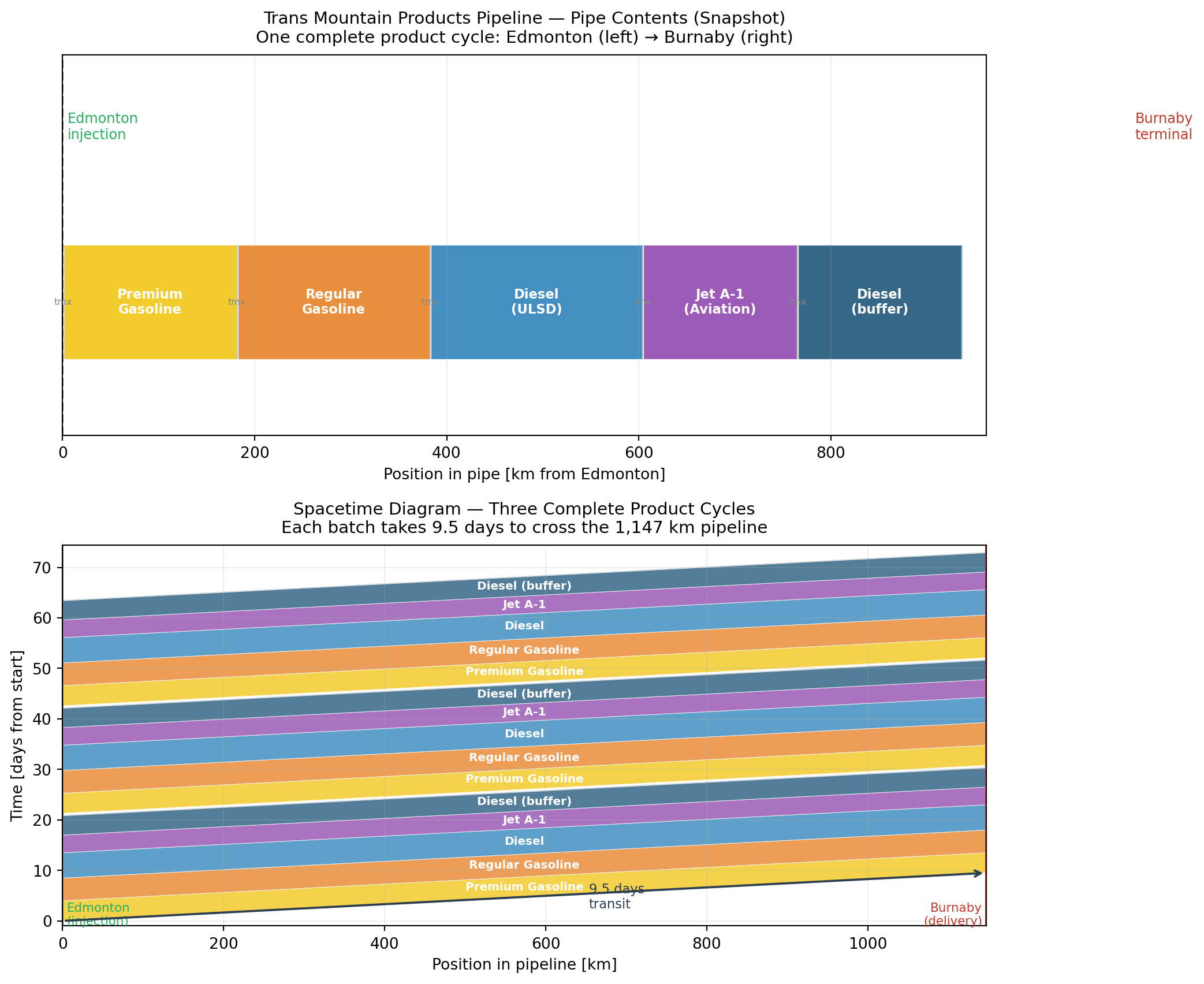
ax1.set_title('Trans Mountain Products Pipeline — Pipe Contents (Snapshot)\n'
              'One complete product cycle: Edmonton (left) → Burnaby (right)',
              fontsize=11, pad=8)
ax1.axvline(1147, color='#c0392b', linewidth=1.5, linestyle='--')
ax1.text(1147, 0.85, 'Burnaby\nterminal', ha='center', va='top',
         color='#c0392b', fontsize=9)
ax1.axvline(0, color='#27ae60', linewidth=1.5, linestyle='--')
ax1.text(5, 0.85, 'Edmonton\ninjection', ha='left', va='top',
         color='#27ae60', fontsize=9)
ax1.grid(axis='x', alpha=0.2)

# ── Bottom: spacetime diagram ─────────────────────────────────────────────────
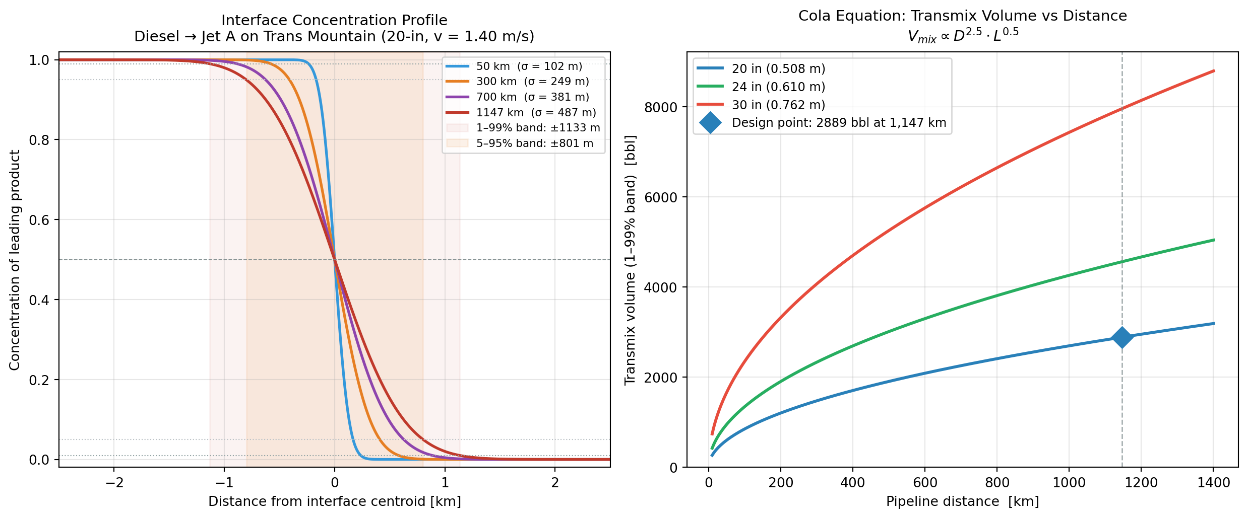
transit_days = 9.5
L_km = 1147.0

# Three cycles of batches
cycle_products = [
    ('Premium Gasoline', '#f1c40f', 4.0),
    ('Regular Gasoline', '#e67e22', 4.5),
    ('Diesel',           '#2980b9', 5.0),
    ('Jet A-1',          '#8e44ad', 3.5),
    ('Diesel (buffer)',  '#1a5276', 3.8),
]
cycle_duration = sum(d for _, _, d in cycle_products) + 0.5

t_inj_start = 0.0
for cycle in range(3):
    t_inj = t_inj_start + cycle * cycle_duration
    for name, col, dur in cycle_products:
        # Injection window: [t_inj, t_inj+dur] at km=0
        # Arrival window at Burnaby: [t_inj+transit, t_inj+dur+transit]
        # Draw parallelogram
        xs = [0, 0, L_km, L_km, 0]
        ys = [t_inj, t_inj + dur, t_inj + dur + transit_days,
              t_inj + transit_days, t_inj]
        ax2.fill(xs, ys, color=col, alpha=0.75, edgecolor='white',
                 linewidth=0.4)
        # Label in centre of parallelogram
        ax2.text(L_km/2, t_inj + transit_days/2 + dur/2, name,
                 ha='center', va='center', fontsize=7.5,
                 color='white', fontweight='bold')

        # transmix (thin grey band)
        xs_tmx = [0, 0, L_km, L_km, 0]
        ys_tmx = [t_inj + dur, t_inj + dur + 0.15,
                  t_inj + dur + 0.15 + transit_days,
                  t_inj + dur + transit_days, t_inj + dur]
        ax2.fill(xs_tmx, ys_tmx, color='#bdc3c7', alpha=0.6, edgecolor='none')

        t_inj += dur

ax2.axvline(0,     color='#27ae60', linewidth=1.5)
ax2.axvline(L_km,  color='#c0392b', linewidth=1.5)
ax2.text(5,    -0.8, 'Edmonton\n(injection)', color='#27ae60', fontsize=8, ha='left')
ax2.text(L_km-5, -0.8, 'Burnaby\n(delivery)', color='#c0392b', fontsize=8, ha='right')

ax2.set_xlim(0, L_km)
ax2.set_ylim(-1, 3 * cycle_duration + transit_days + 1)
ax2.set_xlabel('Position in pipeline [km]', fontsize=10)
ax2.set_ylabel('Time [days from start]', fontsize=10)
ax2.set_title('Spacetime Diagram — Three Complete Product Cycles\n'
              f'Each batch takes {transit_days} days to cross the 1,147 km pipeline',
              fontsize=11, pad=8)
ax2.grid(alpha=0.2)
ax2.annotate('', xy=(L_km, transit_days), xytext=(0, 0),
             arrowprops=dict(arrowstyle='->', color='#2c3e50', lw=1.4))
ax2.text(L_km/2 + 80, transit_days/2, f'{transit_days} days\ntransit',
         ha='left', va='center', fontsize=8.5, color='#2c3e50')

plt.tight_layout()
plt.show()
Figure 2: Top: A snapshot of the Trans Mountain products pipeline pipe contents, showing five product batches plus transmix zones (grey). The sequence — premium gasoline, regular gasoline, diesel, jet fuel, diesel — is governed by contamination compatibility rules (Section 6). Jet fuel requires diesel buffers on both sides; the leading diesel batch prevents upstream gasoline from contaminating the jet A. Bottom: Spacetime diagram showing how three full product cycles traverse the pipeline over 30 days. Each diagonal stripe is a batch injected at Edmonton (left) and arriving at Burnaby (right) after a 9.5-day transit. The transmix zones are the narrow grey boundaries between batches.
import numpy as np
import matplotlib.pyplot as plt

fig, (ax1, ax2) = plt.subplots(1, 2, figsize=(13, 5.5))

# ── Left: inventory simulation ─────────────────────────────────────────────────
D_daily   = 8_000.0   # m³/day diesel demand
t_transit = 9.5       # days
t_cycle   = 5.0       # days between diesel deliveries
t_safe    = 2.0       # safety stock [days]
V_design  = D_daily * (t_transit + t_cycle + t_safe)  # m³

# Thresholds
V_high    = V_design
V_reorder = D_daily * (t_transit + t_safe)    # inject when at this level
V_low_alarm = D_daily * (t_safe * 0.8)         # low alarm
V_stockout  = 0.0

# Simulate
dt     = 0.1        # day step
t_max  = 60.0
t_arr  = np.arange(0, t_max, dt)
V_arr  = np.zeros_like(t_arr)
V_arr[0] = V_design * 0.85   # start partly full

next_delivery = t_cycle      # first delivery at t=5
delivery_vol  = D_daily * t_cycle  # volume of each delivery [m³]

for i in range(1, len(t_arr)):
    t = t_arr[i]
    V = V_arr[i-1] - D_daily * dt   # drawdown
    if t >= next_delivery:
        V = min(V + delivery_vol, V_design)
        next_delivery += t_cycle
    V_arr[i] = max(V, 0)

ax1.plot(t_arr, V_arr / 1000, color='#2980b9', linewidth=2.0,
         label='Diesel inventory')

# Threshold lines
ax1.axhline(V_design / 1000,      color='#27ae60', linestyle='-',
            linewidth=1.2, label=f'High (design capacity — {V_design/1000:.0f} × 10³ m³)')
ax1.axhline(V_reorder / 1000,     color='#f39c12', linestyle='--',
            linewidth=1.3, label=f'Reorder level — injects batch {t_transit:.1f} days early')
ax1.axhline(V_low_alarm / 1000,   color='#e74c3c', linestyle=':',
            linewidth=1.3, label='Low-low alarm')
ax1.axhline(0,                    color='#c0392b', linewidth=0.8)

# Annotate 13-day span
ax1.annotate('', xy=(3.0, V_design/1000), xytext=(3.0, V_reorder/1000),
             arrowprops=dict(arrowstyle='<->', color='#2c3e50', lw=1.3))
ax1.text(4.2, (V_design + V_reorder) / 2000,
         f'Working\ncapacity\n= {t_cycle + t_safe:.0f} days',
         va='center', fontsize=7.5, color='#2c3e50')
ax1.annotate('', xy=(3.0, V_reorder/1000), xytext=(3.0, 0),
             arrowprops=dict(arrowstyle='<->', color='#e74c3c', lw=1.0))
ax1.text(4.2, V_reorder / 2000, f'Transit +\nsafety stock\n= {t_transit + t_safe:.1f} days',
         va='center', fontsize=7.5, color='#e74c3c')

ax1.set_xlabel('Day', fontsize=10)
ax1.set_ylabel('Diesel inventory  [10³ m³]', fontsize=10)
ax1.set_title('Burnaby Terminal — Diesel Inventory Simulation\n'
              f'Demand {D_daily/1000:.0f}k m³/day, delivery every {t_cycle:.0f} days, '
              f'transit = {t_transit} days', fontsize=10, pad=8)
ax1.legend(fontsize=7.5, loc='lower right')
ax1.grid(alpha=0.3)
ax1.set_ylim(-5, V_design / 1000 * 1.15)

# ── Right: required inventory vs transit time ─────────────────────────────────
t_trans_range = np.linspace(0.5, 20.0, 300)
t_cyc_fixed   = 5.0

safety_stocks = [1, 2, 4]
safe_colours  = ['#27ae60', '#f39c12', '#e74c3c']
safe_labels   = ['Safety stock = 1 day', '2 days', '4 days']

for t_s, col, lbl in zip(safety_stocks, safe_colours, safe_labels):
    total_days = t_trans_range + t_cyc_fixed + t_s
    ax2.plot(t_trans_range, total_days, color=col, linewidth=2.2, label=lbl)

# Mark TM scenario
total_TM = t_transit + t_cycle + t_safe
ax2.plot(t_transit, total_TM, 'D', color='#2c3e50', markersize=12, zorder=6,
         label=f'Trans Mountain: {total_TM:.0f} days storage\n(transit {t_transit}, cycle {t_cycle}, safe {t_safe})')
ax2.axvline(t_transit, color='#7f8c8d', linestyle='--', linewidth=1.0, alpha=0.7)
ax2.axhline(total_TM, color='#7f8c8d', linestyle='--', linewidth=1.0, alpha=0.7)

# Reference: hypothetical 2-day transit (truck/barge)
ax2.axvline(2.0, color='#2980b9', linestyle=':', linewidth=1.2, alpha=0.8,
            label='2-day transit (local/barge alternative)')

ax2.set_xlabel('Pipeline transit time  [days]', fontsize=10)
ax2.set_ylabel('Total inventory buffer  [days of supply]', fontsize=10)
ax2.set_title('Required Inventory = Transit + Cycle + Safety\n'
              f'Batch cycle fixed at {t_cyc_fixed:.0f} days', fontsize=11, pad=8)
ax2.legend(fontsize=8, loc='upper left')
ax2.grid(alpha=0.3)
ax2.set_xlim(0, 21)
ax2.set_ylim(0, 32)

plt.tight_layout()
plt.show()
Figure 3: Left: Simulated Burnaby terminal inventory for diesel over 60 days, showing the sawtooth delivery-and-drawdown pattern. Batches arrive every 5 days (averaged across the rotation cycle); between arrivals the tank draws down at constant demand rate. Key inventory thresholds are marked: high (operational ceiling), reorder level (when the next batch must be injected, 9.5 days ahead), low-low alarm, and stockout floor. The 13-day buffer between reorder and high levels is the algebraic result derived in Section 3.5. Right: Required working inventory (in days of supply) as a function of transit time for three safety-stock settings. The Trans Mountain scenario (transit = 9.5 days) is marked; a hypothetical alternative supply with 2-day transit would need only 5–6 days of storage. Geography sets the inventory requirement.

6. Batch Sequencing Rules and Quality Management

The Cola equation tells us how much transmix will form — the sequencing rules tell us how to arrange batches so that the transmix causes minimum quality damage.

Compatibility and the Contamination Direction

Not all product pairs contaminate equally. The critical asymmetry is aviation fuel:

Jet A-1 contaminated by diesel: Aviation fuel (Jet A-1) tolerates a small fraction of diesel contamination — the product’s specification allows fuels of slightly different viscosity and density. The contamination is detectable, the fuel is reclassified, but the safety risk is manageable.

Jet A-1 contaminated by gasoline: Gasoline contamination of aviation fuel is a flight safety critical issue (International Air Transport Association 2023; ASTM International 2024). Gasoline lowers the flash point and changes the combustion characteristics of aviation turbine fuel in ways that can affect engine performance. The contamination threshold is extremely low — even 1% gasoline contamination by volume requires the batch to be rejected or extensively retested. An aviation fuel batch cannot be adjacent to a gasoline batch in the pipeline without a buffer.

Diesel contaminated by gasoline: Road diesel contaminated with gasoline reduces the cetane number and flash point. Small contamination percentages (2–5%) are tolerable in some specifications but must be tested and documented. The contamination is operationally managed, not a safety incident.

Gasoline grades adjacent to each other: Premium and regular unleaded gasoline batches adjacent to each other produce transmix that falls between the two grades — typically reclassified as regular or blended with other regular batches. This is the most benign interface.

The Canonical Sequencing Rule

The standard sequencing for a multi-product pipeline carrying gasoline, diesel, and jet fuel is:

\underbrace{\text{Premium gasoline}}_{\text{upstream}} \to \underbrace{\text{Regular gasoline}}_{\text{any sequence with premium}} \to \underbrace{\text{Diesel}}_{\text{compatibility buffer}} \to \underbrace{\text{Jet A-1}}_{\text{protected both sides}} \to \underbrace{\text{Diesel}}_{\text{back-buffer}} \to \underbrace{\text{Regular gasoline}}_{\text{next cycle}}

The diesel batches on both sides of jet fuel serve as cushion batches: they absorb the gasoline/diesel transmix on the upstream side and the diesel/jet transmix on the downstream side, ensuring that no gasoline molecules reach the aviation fuel. The cushion diesel batch may itself become off-specification — a diesel/gasoline transmix — and is managed by cutting and blending at the terminal.

Interface volume accounting for a jet fuel batch:

  1. Gasoline upstream → diesel cushion interface: Cola volume of gasoline/diesel transmix
  2. Diesel cushion → jet fuel interface: Cola volume of diesel/jet transmix (this enters the jet batch from the front)
  3. Jet fuel → diesel back-buffer interface: Cola volume of jet/diesel transmix (this exits the jet batch at the rear)
  4. Diesel back-buffer → next gasoline interface: Cola volume of diesel/gasoline transmix

The jet fuel batch must be sized to deliver the contracted volume after removing the two Cola volumes at its leading and trailing edges. The cushion diesel batches must be sized to absorb their gasoline interfaces and still deliver usable diesel — or the cushion volume is explicitly written off as interface loss.

Cut Point Decisions at the Terminal

At Burnaby, trained operators monitor the arrival of each interface using densitometers and chromatographic analysers inline on the receiving header. As the interface arrives, the product switches at a precisely calculated cut point — the moment at which the flow is redirected from the on-specification tankage to the transmix tank or the off-specification blend tank.

The cut point decision trades off two risks: - Cutting too early (at a concentration above specification): some on-specification product is diverted to the transmix tank, reducing yield. - Cutting too late (below specification threshold): contaminated product enters the on-specification tank, potentially requiring reclassification of the entire tank’s contents.

For aviation fuel, there is no “cutting too late” — the cut is always conservative (early), accepting some yield loss to guarantee that no contaminated fuel reaches the aviation specification tank. For road fuels, the cut point optimises for maximum on-specification yield within the product’s contamination tolerance.


7. The Edmonton to Burnaby Pipeline: A Case Study

The Trans Mountain products pipeline service — the original 20-inch pipeline built in 1953, now supplemented by the 2024 expansion — carries approximately 150,000–200,000 barrels per day of refined products from Edmonton refineries (primarily Imperial Oil’s Strathcona Refinery and Suncor’s Edmonton refinery) to Metro Vancouver and coastal British Columbia (Trans Mountain Corporation 2024; Canada Energy Regulator 2024).

Pipeline geometry: 1,147 km from Edmonton to Burnaby, diameter 20 inches (508 mm) for the majority of the route. The terrain crosses the Rocky Mountains through the Rogers Pass corridor, with elevation changes of up to 1,000 metres. Unlike the flat prairie corridors of P1 and P3, the Trans Mountain products line must manage significant elevation head: uphill sections require more pump pressure; downhill sections must be controlled to avoid overpressure or flow runaway (a phenomenon called “slack line” where the downhill section operates at atmospheric pressure if pump pressure is reduced too much).

Product slate: The Edmonton refineries produce gasoline (regular and premium), diesel, jet fuel (Jet A-1), aviation gasoline (AVGAS), and heating oil (furnace fuel). Not all products move through the pipeline at all times; the mix depends on seasonal demand, refinery production rates, and terminal inventory levels. Summer demand favors gasoline; winter shifts toward heating oil and diesel.

Burnaby terminal: The Trans Mountain terminal at Burnaby, on Burrard Inlet, has approximately 13 days of total petroleum storage for Metro Vancouver. Products transfer from the terminal to retail distributors by truck rack; aviation fuel travels by a dedicated pipeline to Vancouver International Airport. Marine fuel (bunker C and marine diesel) is loaded directly to bunker barges from the terminal’s marine dock.

The 2018 spill and supply implications: In November 2018, a spill at the Burnaby terminal forced a 90-day shutdown of products delivery. During this period, Metro Vancouver’s refined products supply fell to truck transport from Alberta (limited capacity) and imports through the Westridge marine terminal (normally used for crude oil exports). The inventory buffer — approximately 13 days — provided the window for emergency supply measures to mobilize. This episode validated the inventory design: 13 days was sufficient to prevent acute supply disruption, but barely (Canada Energy Regulator 2024).


8. Interpretation

The D^{2.5} penalty for larger-diameter products pipelines

The Cola equation’s D^{2.5} diameter dependence has a design implication that does not arise for crude oil or gas transmission: for refined products, increasing pipe diameter to increase capacity also proportionally increases transmix volume and therefore interface losses. A 30-inch products pipeline produces approximately (30/20)^{2.5} = 1.5^{2.5} \approx 2.76 times as much transmix per interface as a 20-inch pipeline carrying the same length of route.

This means that the transmix management cost — the write-off of interface material to reprocessing — scales superlinearly with pipe diameter. Large-diameter crude oil pipelines do not face this penalty because crude oil is a single undifferentiated product (within grade); large-diameter gas pipelines do not face it because natural gas is a single commodity. Refined products pipelines are unique in having an operating cost that grows with pipe diameter beyond the capacity benefit.

In practice, this creates an incentive to keep batch sizes large (reducing the interface-to-volume ratio) and to invest in interface detection and blending infrastructure at receiving terminals rather than in ever-larger pipeline diameters.

Transit time is geography’s invoice

The inventory design equation makes a simple statement about geography: the farther the terminal is from the refinery, the more inventory it must hold. There is no operational workaround. Edmonton’s refineries can respond to Vancouver demand signals only with a 9.5-day delay. That delay is not a policy choice or a market failure — it is the solution to L/v = 1{,}147{,}000 / 1.40 = 819{,}285 seconds = 9.48 days, which is physics and geography, not regulation.

The 2003 Imperial Oil pipeline curtailments, the 2018 Burnaby terminal spill, and the winter 2022 cold-snap demand surge all demonstrated the same mathematics in market terms: Metro Vancouver has limited ability to quickly substitute for Trans Mountain products supply because no alternative source can cover 1,147 km of pipeline distance in under nine days by any other means. Barge and ship are slower; truck is capacity-limited. The transit time is, in the most literal sense, geography’s invoice for locating a major coastal city behind a mountain range.


9. What Could Go Wrong

Elevated transmix volumes from DRA (drag-reducing agent) injection

P1 noted that crude oil pipelines routinely inject drag-reducing agents to increase throughput beyond Darcy-Weisbach predictions. Products pipelines also use DRA — but DRA injection at batch interfaces changes the local flow regime in ways that can increase transmix beyond the Cola equation prediction. DRA polymers degrade through pump impellers, creating concentration gradients that interact with the interface dispersion. Pipeline operators typically avoid injecting DRA immediately upstream of product interfaces, accepting some throughput reduction during interface transit to maintain Cola-equation-level transmix volumes.

Aviation fuel contamination incident protocol

An aviation fuel batch arriving at Burnaby below specification triggers a full emergency protocol: the batch is diverted to the transmix tank, all aircraft that may have received product from the suspect batch are grounded for tank draining and re-inspection, and the airport switches to emergency fuel reserves while the pipeline clears and redelivers a confirmed on-specification batch. The Transit time from Edmonton means that a suspected contamination event at the refinery requires 9.5 days to resolve through new product delivery — a long window for aviation operations disruption (International Air Transport Association 2023).

This is why batch certification practices at Edmonton are strict: the cost of a contamination event (lost flights, aircraft grounding, emergency fuel procurement) far exceeds the cost of conservative quality management at the injection point.

Slack line in the Rocky Mountain descent

On the descent from the Rocky Mountain summit toward the Lower Mainland, the Trans Mountain products pipeline encounters negative elevation change of roughly 1,000 metres over 150 km. If the flow is slowed (reduced pump rate, maintenance valve throttling), the downhill sections can enter slack line conditions: the pipe pressure at the valley floor falls below the liquid’s vapor pressure at that point, creating vapor pockets. When pressure is restored and the vapor pockets collapse, the resulting pressure surge can exceed the pipe’s maximum allowable operating pressure — a hydraulic hazard.

Operating procedures for the descent section require maintaining minimum flow rates and monitoring pressure profiles carefully during any pump startup or shutdown sequence. The elevation correction term (\rho g \Delta z) that P1 mentioned briefly is fully load-bearing here: it modifies the pressure budget in the downhill direction by +10 MPa for a 1,000-metre descent in diesel — more than the pump pressure the stations provide. Managing this is one of the most complex aspects of Trans Mountain products pipeline operation.

Demand pattern shifts and batch cycle economics

The Trans Mountain products schedule is planned months in advance based on refinery production forecasts and terminal inventory targets. A sudden demand shift — a cold snap increasing heating oil demand, a summer driving surge, or a large industrial customer outage — disrupts the planned batch sequence. The pipeline cannot respond faster than its transit time; the terminal must manage through its working inventory. If the demand shift exceeds the safety stock buffer, the terminal approaches low-alarm thresholds and emergency sourcing (coastal imports, truck from other terminals) must be activated.


10. Extension: Pump Power and Products Pipeline Economics

The products pipeline economics differ from crude oil and gas in one important way: tariff recovery per unit volume must compete with trucking, which sets a market ceiling on pipeline tariffs at shorter distances.

Within Alberta, refined products trucking from Edmonton is economically competitive for deliveries within approximately 400 km. Beyond 400 km — which includes most of BC’s interior and all of the coast — pipeline is cost-competitive. The Trans Mountain products tariff of approximately CAD 5–7 per cubic metre for the full Edmonton–Burnaby route is substantially below the equivalent trucking cost of CAD 50–80/m³ for that distance. The pipeline’s capital cost, amortised over decades of throughput, produces a per-unit tariff that trucking can never match at this distance.

The pump station energy cost for the products pipeline is calculated exactly as in P1:

P_{\text{pump}} = \frac{Q \cdot \Delta P}{\eta}

For the Trans Mountain products line at Q = 0.277 m³/s (150,000 bbl/day) and a total pressure budget of approximately 60 MPa across all stations:

P_{\text{pump}} = \frac{0.277 \times 60 \times 10^6}{0.82} \approx 20.3 \;\text{MW total}

distributed across approximately 12 pump stations from Edmonton to Burnaby. Annual energy cost at CAD 0.08/kWh: 20.3 \times 10^3 \;\text{kW} \times 8{,}760 \;\text{hr/yr} \times 0.08 \approx \text{CAD }14.3 \;\text{million/yr}

Divided across 150,000 bbl/day × 365 days = 54.75 million bbl/yr: \text{CAD }14.3\text{M} / 54.75\text{M bbl} \approx \text{CAD }0.26/\text{bbl energy cost}

The energy component of the tariff is modest — the dominant cost is capital amortization on a $2+ billion pipeline and pump station infrastructure.


11. Math Refresher: The Error Function and \sqrt{L} Scaling

Why diffusion grows as \sqrt{L}

The concentration profile at a batch interface follows the error function family because the underlying process — turbulent dispersion — is a random walk. Each small element of fluid makes random lateral jumps due to turbulent eddies, and the net longitudinal displacement accumulates statistically. In a random walk of N steps of size \ell, the standard deviation of displacement is \ell \sqrt{N} — not N\ell. The steps add in quadrature, not in sum.

In a pipeline of length L at velocity v, the transit time is t = L/v. If turbulent eddies make jumps of characteristic time scale \tau_c, the number of independent mixing events is N = t/\tau_c = L/(v \tau_c). The standard deviation of the interface position therefore grows as:

\sigma \propto \sqrt{N} \propto \sqrt{L}

This is why the Cola equation has L^{1/2}, not L^1: diffusive processes always produce the square root.

The complementary error function

The interface concentration profile is: c(x) = \frac{1}{2}\operatorname{erfc}\!\left(\frac{x}{\sqrt{2}\,\sigma_x}\right)

The complementary error function \operatorname{erfc}(z) = 1 - \operatorname{erf}(z) where \operatorname{erf}(z) = (2/\sqrt{\pi})\int_0^z e^{-t^2}\,dt.

Key values:

\operatorname{erf}(z) c at this x = z\sqrt{2}\,\sigma_x Band
0.84 \frac{1}{2}(1 - 0.84) = 0.08 8%
0.95 \frac{1}{2}(1 - 0.95) = 0.025 2.5%
0.98 \frac{1}{2}(1 - 0.98) = 0.01 1%

The 1% cutoff corresponds to z = \operatorname{erfinv}(0.98) \approx 1.645, so x_{1\%} = 1.645\sqrt{2}\,\sigma_x = 2.326\,\sigma_x on each side of the interface.

Connecting back to pipeline design

The Cola equation’s D^{5/2} L^{1/2} scaling makes transmix a quantity that engineers can control through two levers: - Diameter: specified at the design stage and essentially unchangeable afterward — choose smaller diameter to reduce transmix per interface, accepting lower throughput - Distance: fixed by geography — cannot be reduced, but can be accommodated through larger batches and more terminal storage

The L^{1/2} growth means that terminal storage grows only as \sqrt{L}, not as L — a natural moderating factor. Doubling the pipeline length increases transmix by only 41%, not 100%. The inventory design, by contrast, grows linearly with transit time: a pipeline twice as long requires twice the storage buffer. Of the two penalties for distance — more transmix and more storage — the storage penalty is steeper.


Summary

Concept Key equation What it governs
Taylor dispersion coefficient K = 10.1\, r_0\, u^* Apparent longitudinal diffusivity in turbulent pipe flow
Shear velocity u^* = v\sqrt{f/8} Turbulence intensity near the wall
Interface standard deviation \sigma_x = \sqrt{2KL/v} Width of dispersion zone at distance L
Concentration profile c(x) = \tfrac{1}{2}\operatorname{erfc}(x/\sqrt{2}\sigma_x) Product fraction at any position in interface
Cola equation V_{mix} = 6.91\,f^{1/4}\,D^{5/2}\,L^{1/2} Transmix volume (1–99% band)
Minimum batch size V_{batch} = V_{delivery} + 2V_{mix} Batch injection volume for contracted delivery
Working inventory V_{working} = D_d \times (t_{cycle} + t_{safe}) Tank drawdown between deliveries
Design inventory V_{design} = D_d \times (t_{transit} + t_{cycle} + t_{safe}) Total tank size from pipeline physics

The physical result that matters most: Transmix grows as the square root of pipeline distance and the 2.5th power of pipe diameter. These two scaling relationships set a hard floor on interface losses on any multi-product pipeline: losses cannot be eliminated by operating practice, only managed. The batch sequencing rules exist to ensure that unavoidable transmix contaminates the least critical product interfaces first.

The economic result that matters most: The terminal inventory design equation reveals that the Burnaby terminal’s thirteen-day buffer is not a regulatory prescription or a commercial choice — it is the algebraic output of a 9.5-day pipeline transit time, a 5-day average batch cycle, and a 2-day safety stock. Geography set the transit time; the transit time set the inventory; the inventory set the tank farm. A shorter pipeline would require smaller tanks; no such pipeline exists.


Next: P5 — The Integrated Network — all four commodity systems as a directed graph, max-flow min-cut analysis, network centrality, and the full netback price surface across all market destinations.

References

ASTM International. 2024. ASTM D1655: Standard Specification for Aviation Turbine Fuels. ASTM International. https://www.astm.org/.
Canada Energy Regulator. 2024. Pipeline Profiles. Canada Energy Regulator. https://www.cer-rec.gc.ca/en/data-analysis/infrastructure/pipeline-profiles/.
Cola, R. 1965. “Contamination Length of Two Adjacent Batches of Different Petroleum Products Flowing in a Pipeline.” L’Energia Elettrica 42: 753–62.
Imperial Oil Limited. 2024. Annual Report 2024. Imperial Oil Limited. https://www.imperialoil.ca/en-CA/Investors/Financial-information.
International Air Transport Association. 2023. IATA Guidance Material for Aviation Turbine Fuels Specifications. 9th ed. International Air Transport Association. https://www.iata.org/.
Menon, E. Shashi. 2015. Transmission Pipeline Calculations and Simulations Manual. Gulf Professional Publishing. https://doi.org/10.1016/C2013-0-13698-8.
Taylor, G. I. 1954. “The Dispersion of Matter in Turbulent Flow Through a Pipe.” Proceedings of the Royal Society of London. Series A 223 (1155): 446–68. https://doi.org/10.1098/rspa.1954.0130.
Trans Mountain Corporation. 2024. Trans Mountain Expansion Project: In-Service Announcement. Trans Mountain Corporation. https://www.transmountain.com/expansion-project.
Back to top